Why Trade Results Are Better Understood as Distributions
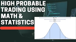
Most people approach trading by asking a single question: what will happen on the next trade? A probability-based approach replaces that question with a different one: what does the full set of outcomes look like when a system is repeated many times? The core idea behind any probability distribution chart is simple. The center of the chart represents the average or most typical result. The further a value sits from that center, the less frequently it occurs. Nothing about this requires advanced mathematics. If a trader collects enough sample data, groups the results into value ranges, and counts how often each range appears, a bar chart of frequencies emerges on its own. The same method applies directly to a trading system. Instead of forecasting which individual trade will win or lose, the trader records the outcome of every trade over a long period and sorts those outcomes into buckets. The resulting shape describes the behavior of the system as a whole. Two properties of that shape matter most: where the mass of outcomes is concentrated, and how far the tails extend on each side. One important caveat is sample size. A distribution built from ten or twenty trades is unstable and often misleading, because random variation dominates. Only with a large sample does the underlying shape become visible and reasonably repeatable. A second caveat is purpose. A distribution chart is a description of past system behavior across many repetitions. It is not a forecast of the next outcome, and treating it as one is one of the most common misuses of the tool. The value of the approach lies in understanding what the system normally produces and how often extreme outcomes appear.
Building the Picture from Sample Data
Constructing a useful distribution begins with choosing a measurement unit. Three common choices are the percentage return of a period, the dollar profit or loss of a trade, and the R-multiple. The R-multiple normalizes every trade by the amount of risk that was committed at entry, which makes trades of different sizes and different markets directly comparable. If a trade risked one unit of capital at entry, a loss of that unit is minus one R, a gain twice that size is plus two R, and so on. The mechanical steps are straightforward. First, define the risk unit consistently so that every trade is measured on the same scale. Second, record the result of each closed trade in R-multiples. Third, group the results into intervals, for example bands of half an R or one R. Fourth, count how many trades fall into each band. Fifth, plot the counts as bars. The same procedure works for monthly returns, where each month is measured as a percentage and the bands might be one or two percentage points wide. A few practical details affect how readable the chart is. The number of buckets should be large enough to reveal shape but not so large that every bar is nearly empty. The sample should cover a long enough period to include different market environments, since a shape drawn only from a strong trending period may look very different from one drawn across a full cycle. Results from a backtest and results from live trading may also differ, because real execution includes slippage, partial fills, and human decisions that a simulation may not capture. Finally, the chart should be read as an estimate rather than a fixed law. It summarizes what a system has produced, and its stability can only be judged by comparing distributions across different time windows and market conditions.
Monthly Returns: A Roughly Normal Shape with a Longer Right Side
A long-running trend following system, measured by monthly percentage returns, often produces a histogram that resembles a normal distribution at first glance. Most months cluster near the center, which may sit close to zero or slightly positive, and the frequency falls off as returns move away from that center in either direction. However, there is usually one clear difference from a symmetrical bell curve: the right side stretches further out. A few months deliver returns that are much larger than the typical month, pushing the positive tail far to the right. Statisticians describe this as positive skew, and the extended right side is often called a fat tail. The practical meaning is that the bulk of results are unremarkable while a small number of periods account for a disproportionate share of total performance. This pattern is closely related to how trends behave. Markets frequently move sideways or oscillate for extended periods, producing modest and inconsistent results. Occasionally, a sustained directional move develops and a system that holds positions through it can capture an unusually large gain. It is worth noting that monthly aggregation tends to smooth the picture. Losses on the left side may look limited because risk controls cap how much a single position can lose, while gains on the right remain open-ended. The same system viewed at the level of individual trades usually shows a much more dramatic asymmetry than the monthly chart suggests. The main misuse here is expecting a typical month to be representative. Judging a system by a short window of monthly returns, whether good or bad, tends to produce conclusions that the full distribution does not support. Performance arrives unevenly, and the distribution is the record of that unevenness.
The R-Multiple Distribution of Individual Trades
At the level of single trades, the shape becomes more extreme. In a trend following approach, losing trades typically outnumber winning trades by a substantial margin. This is not a sign that something is broken. It is a direct consequence of trying to participate in rare, large moves: most attempts to enter a trend fail, and each failure is closed quickly with a small loss. On the losing side of the histogram, the bars cluster heavily near minus one R, meaning most losses end close to the initial risk commitment rather than far beyond it. The winning side looks entirely different. There are fewer trades there, and the bars are spread across a wide range. Some winners end slightly above break-even, others produce one or two R, and a small number extend to several times the initial risk. In rare cases a single trade can produce a result many multiples of the original risk. The distribution therefore has a dense cluster on the left near minus one R, a sparse and thin scattering on the right, and a long extension into large positive values. The system logic is embedded in this shape. By holding each loss to roughly the initial risk, the left side stays tightly bounded. By allowing winners to remain open as long as the trend persists, the right side is left unbounded. The arithmetic that follows is that a small number of large winners can offset a much larger number of small losses and still leave a net surplus. This also explains why win rate alone carries little information. A system with a high win rate but a short right tail may be fragile, while a system with a low win rate and a long right tail may be robust in a trending environment. A common misuse is to raise the win rate by taking profits early, which shortens the right tail and alters the very shape the system depends on.
How System Rules Shape the Distribution
The distribution of results is not an accident. It is largely determined by the rules that govern entries, exits, and position sizing. The risk per trade, decided before entry and enforced by a stop, defines the one R unit and caps the loss on the left side. The exit logic for profitable positions determines how far the right tail can extend. A trailing stop or a trend-following exit that stays in a position while the trend continues allows a winner to grow well beyond the initial risk. Combine a hard cap on losses with an open-ended exit on gains, and the asymmetric R-multiple distribution follows from the design itself. This also means the shape is conditional on the environment. Trends do not appear on schedule. In a market that oscillates for a long stretch without producing sustained directional moves, the large winners that populate the right tail become rare. The many small losses on the left side continue to accumulate, and the system can enter a net negative phase. That outcome reflects the environment rather than a broken rule set. Understanding this helps separate two very different problems: a distribution behaving as designed in an unfavorable regime, and a distribution that has genuinely shifted because the rules are being applied inconsistently. Execution quality belongs in the same discussion. A stop that is widened mid-trade, a position that is closed early out of discomfort, or a winner that is abandoned before the trend ends all modify the distribution. Each such decision tends to clip the right tail or widen the left, moving the shape away from what the rules were meant to produce. In that sense, the histogram is not only a record of market behavior; it is also a record of how faithfully the process was followed, which is why comparing planned and realized distributions can be informative.
Probability Density: How Often a Specific Outcome Appears
Probability density answers a narrow question: how concentrated are outcomes around one particular value? Picture a smooth curve drawn over the histogram. The height of that curve at any point represents how frequently results land near that value. A high point means the outcome is common; a low point means it is rare. In the R-multiple distribution of a trend following system, the highest point on the curve usually sits near minus one R. In plain terms, the single most likely result of any given trade is a loss that stays within the initial risk. This has a direct psychological implication. Frequent small losses are not evidence of a malfunction; they are the most probable outcome by construction. The design accepts many small failures in exchange for the possibility of rare large gains. A trader who understands the density curve is less likely to reinterpret a normal losing streak as a reason to change the rules. A useful analogy comes from everyday life. Probability density is like asking how likely it is to meet a person whose height is exactly a given value. It is a point concept: it describes the concentration of probability at one specific number. The same idea applies to trades. The density curve does not say anything about the total risk of a sequence of trades, and it does not indicate how much could be lost across a month or a year. It only describes which single outcomes occur most often. Confusing this point-level view with a range-level view is one of the most common errors when reading a distribution, and it is the reason the next concept is needed alongside it.
Cumulative Probability: How Much Loss the Worst Cases Carry
Cumulative probability answers a different question: what is the total chance that a result falls at or below a given value? Visually it is a curve that starts near zero at the far left and rises toward one hundred percent at the far right. At any point on the horizontal axis, the height of the curve represents the proportion of all outcomes that are no larger than that value. If the cumulative probability reaches ninety-five percent at a particular loss level, it means that ninety-five percent of results lose no more than that amount. Only five percent are worse. The same analogy from before applies. If probability density is the chance of meeting a person of exactly a given height, cumulative probability is the chance of meeting a person no taller than a given height. It is a range concept rather than a point concept. In evaluating a trading system, this view is used to estimate how deep adverse results can go. It supports thinking about the size of capital reserves that a given loss profile would require, and about how much psychological tolerance an extended losing sequence would demand. There are important limitations. Cumulative probability for single trades cannot simply be added up to produce cumulative probability for a sequence of trades, because outcomes are not independent in practice and because the order of results matters for equity drawdowns. Sequence-level questions, such as the probability of a drawdown exceeding a certain percentage, usually require simulation or analysis of actual sequence data. There is also the problem of estimation: the extreme tails are by definition rare, so any estimate of them rests on a limited number of observations and can shift considerably when new data arrives. The cumulative view is therefore best treated as an approximate map of risk rather than a precise guarantee.
The Turtle Mindset: Evaluating the System, Not the Trade
The Turtle traders approached every trade from a probability standpoint. They could not know whether a specific trade would make or lose money. What they knew was the shape of the distribution their system produced: many small losses near one R, a smaller number of moderate gains, and a rare few trades with outsized profits. That knowledge, rather than any forecast of the next trade, was the basis for taking each position. Accepting that the most likely outcome of any single trade is a loss changes how results are interpreted. A loss is not a personal failure; it is a normal and necessary cost of running the system. A gain is not proof of skill; it is an expected part of the right tail. Because evaluation is attached to the distribution rather than to the individual trade, the emotional weight of any one outcome is reduced. That reduction is what makes consistent execution possible over long sequences that include many losses before a large winner appears. This mindset does not remove uncertainty or risk. It aligns expectations with what the system actually produces, so that a normal losing streak does not trigger rule changes and a single large win does not trigger overconfidence. The two analytical tools described earlier support this stance. Probability density identifies the outcome that will occur most often and normalizes the frequent small loss. Cumulative probability quantifies how far the adverse side can extend and informs how much capital and tolerance may be needed. Together they form a complete framework for understanding a trading system through the lens of probability rather than through the outcome of the last trade. Based on study notes, for educational purposes only and not investment advice.